Benchmark Functions

This page documents the benchmark tests used to validate the BOAR optimization framework. Two classic optimization test functions are used: Ackley and Rosenbrock. Followed by a constrained version of each function to demonstrate the framework’s ability to handle constraints. Lastly a BASEMENT benchmark is included to demonstrate the framework’s ability to handle a two-dimensional hydrodynamic models calibration.

Ackley Function

The Ackley function is a non-convex function commonly used to test optimization algorithms. It has many local minima but one global minimum.

Function Definition

\[f(x, y) = -20 \exp\left(-0.2 \sqrt{\frac{x^2 + y^2}{2}}\right) - \exp\left(\frac{\cos(2\pi x) + \cos(2\pi y)}{2}\right) + e + 20\]

Properties

Property	Value
Global Minimum	0 at (0, 0)
Search Domain	[-32.768, 32.768]
Difficulty	Multi-modal, many local minima

Optimization configurations (Ackley)

optimization_variable_options:
  'bounds': [!!python/tuple [-32.768, 32.768]]
  'precision': None
  'n_initial': 15

surrogate_model_options:
  'max_tested_vectors': 100
  'tolerance': 1e-6
  'GPR_iterations': 500
  'test_population': 100000

sampling_options:
  'seed': 9

Benchmark Results

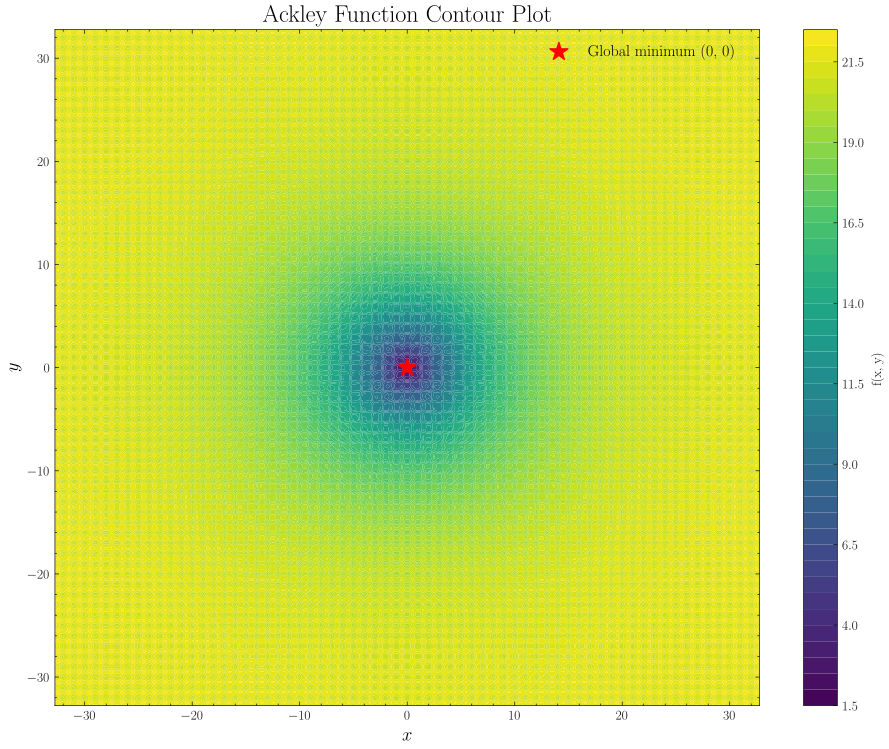
Figure 1: Contour plot of the 2D Ackley function showing global minimum at center.

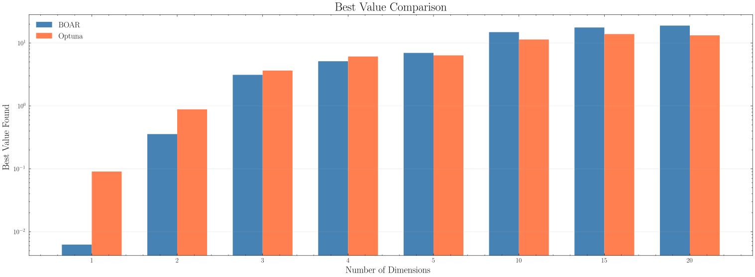
Figure 2: Comparison of available BOAR optimization results on the Ackley function.

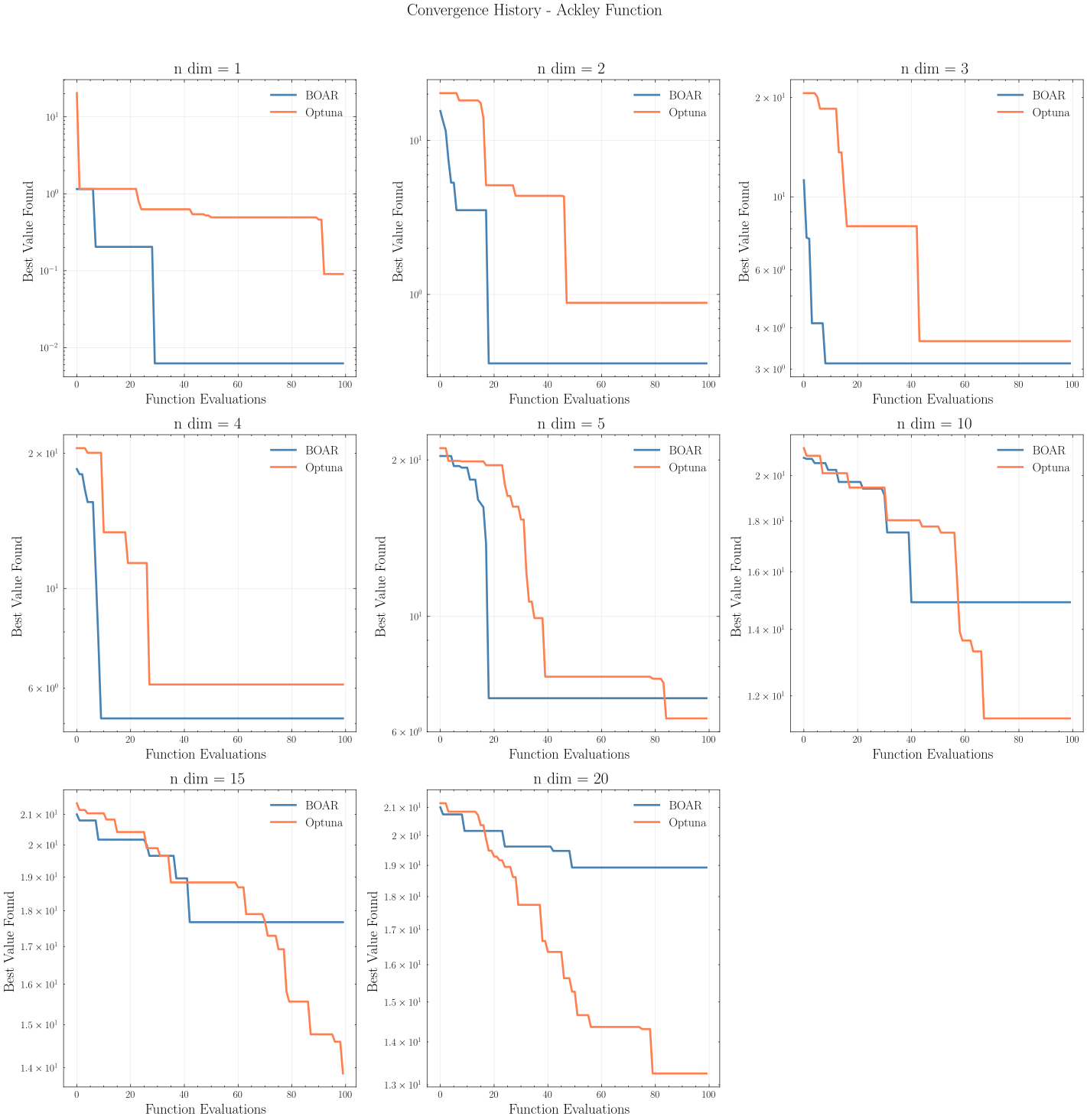
Figure 3: BOAR optimization convergence on the Ackley function.

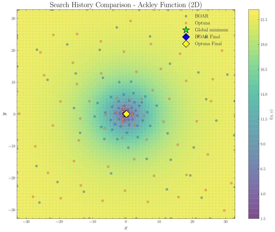
Figure 4: Search history of BOAR optimization on the 2D Ackley function.

Constrained version

The Ackley function can also be tested with constraints, such as limiting the search space to a specific region or adding inequality constraints. In this test case, we defined the following constraint:

\[g(x, y) = x_i + x_{i+1} + \ldots + x_n \leq 0\]

This constraint limits the sum of the optimization variables, creating a more challenging optimization problem.

Constrained Benchmark Results

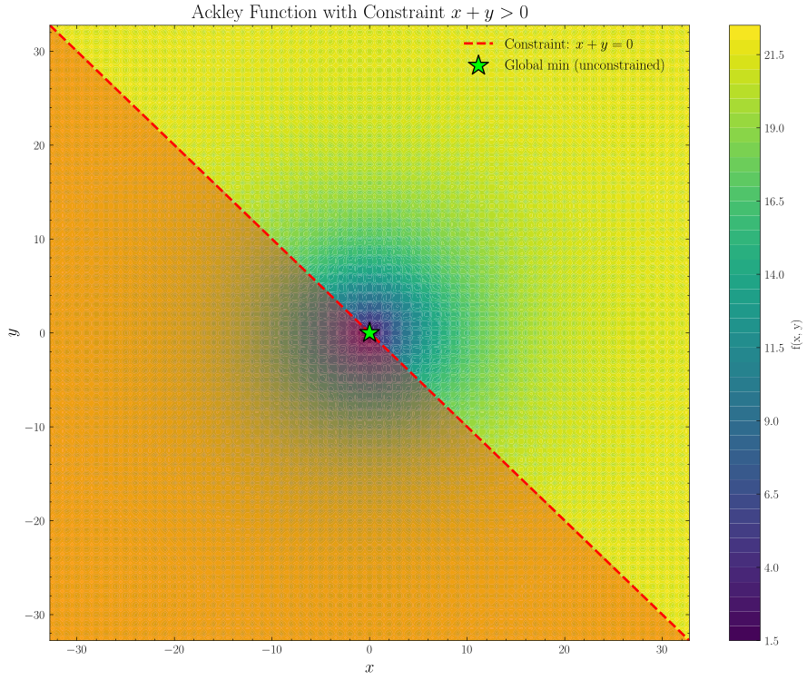
Figure 5: Contour plot of the 2D constrained Ackley function showing feasible region.

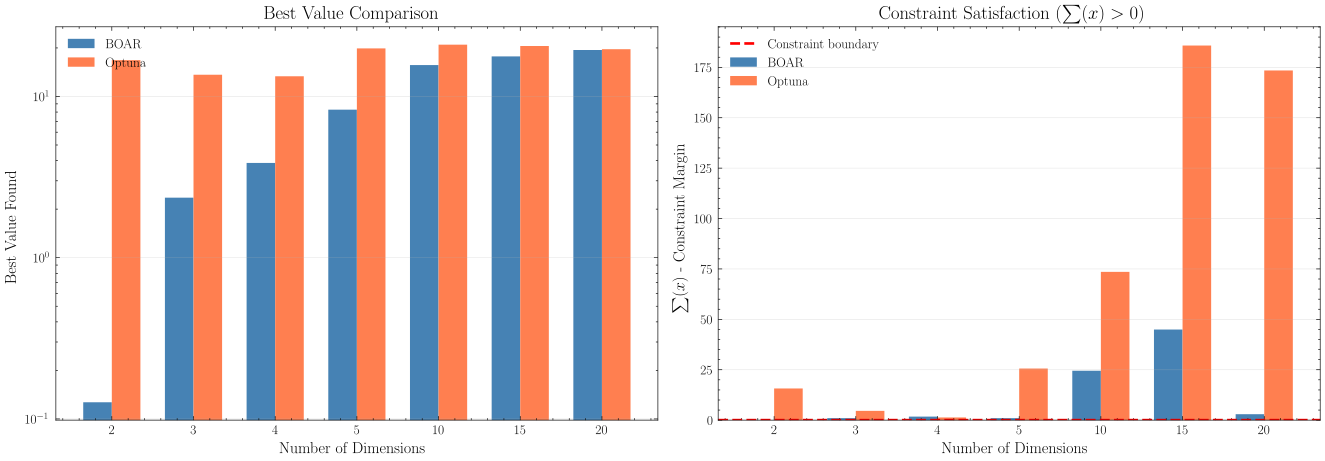
Figure 6: Comparison of available BOAR optimization results on the constrained Ackley function.

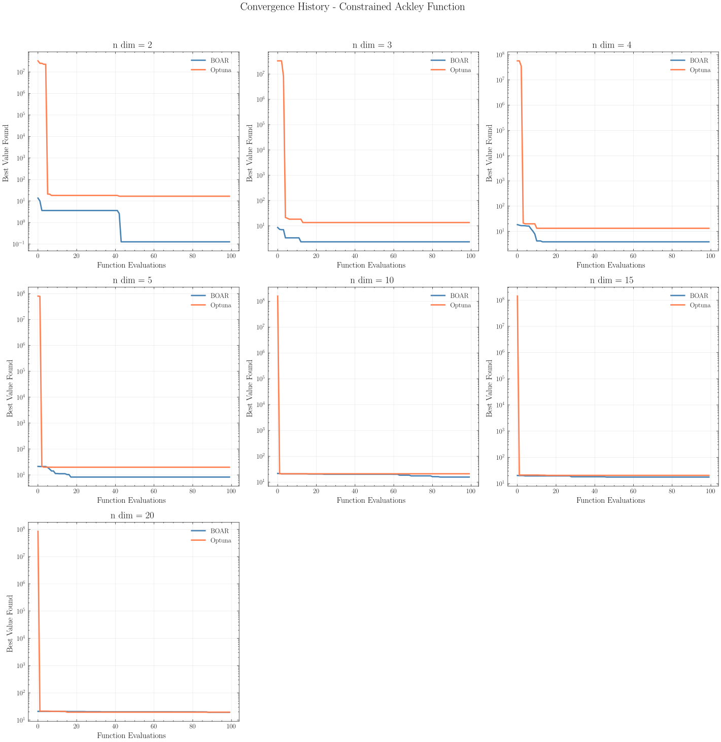
Figure 7: BOAR optimization convergence on the constrained Ackley function.

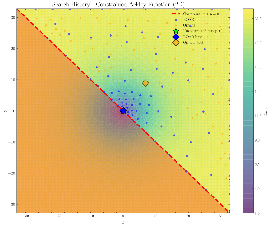
Figure 8: Search history of BOAR optimization on the 2D constrained Ackley function.

Rosenbrock Function

The Rosenbrock function is a non-convex function commonly used to test optimization algorithms. It has many local minima but one global minimum.

Function Definition

\[f(x, y) = (a - x)^2 + b(y - x^2)^2\]

Properties

Property	Value
Global Minimum	0 at (1, 1)
Search Domain	Typically [-5, 10]
Difficulty	Narrow curved valley, hard to optimize

Optimization configurations (Rosenbrock)

optimization_variable_options:
  'bounds': [!!python/tuple [-5, 10]]
  'precision': None
  'n_initial': 15

surrogate_model_options:
  'max_tested_vectors': 100
  'tolerance': 1e-6
  'GPR_iterations': 500
  'test_population': 100000

sampling_options:
  'seed': 9

Benchmark Results

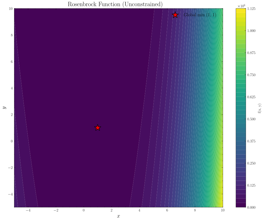
Figure 9: Contour plot of the 2D Rosenbrock function showing global minimum at (1, 1).

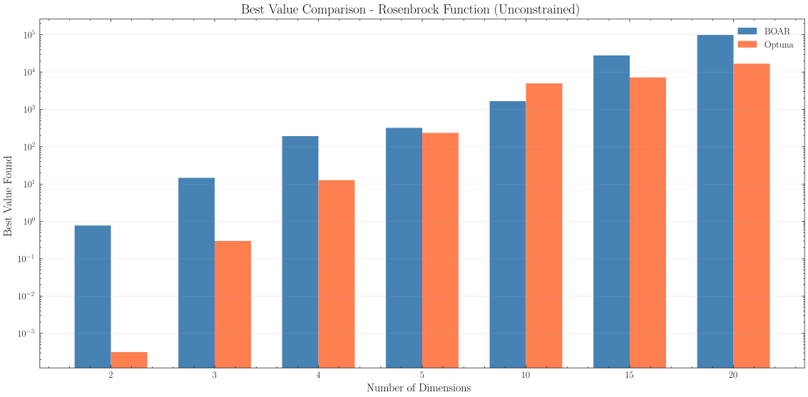
Figure 10: Comparison of available BOAR optimization results on the Rosenbrock function.

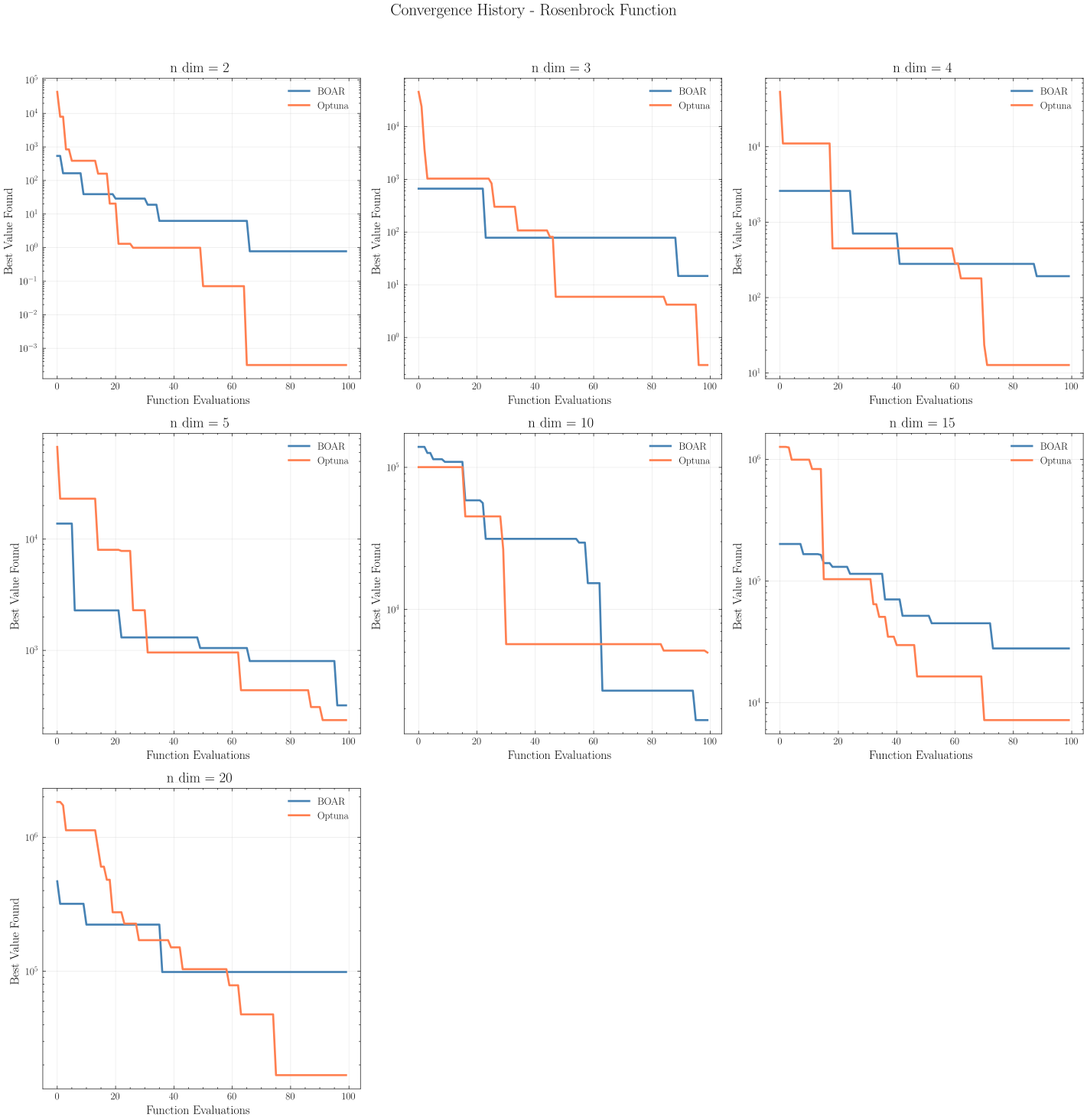
Figure 11: BOAR optimization convergence on the Rosenbrock function.

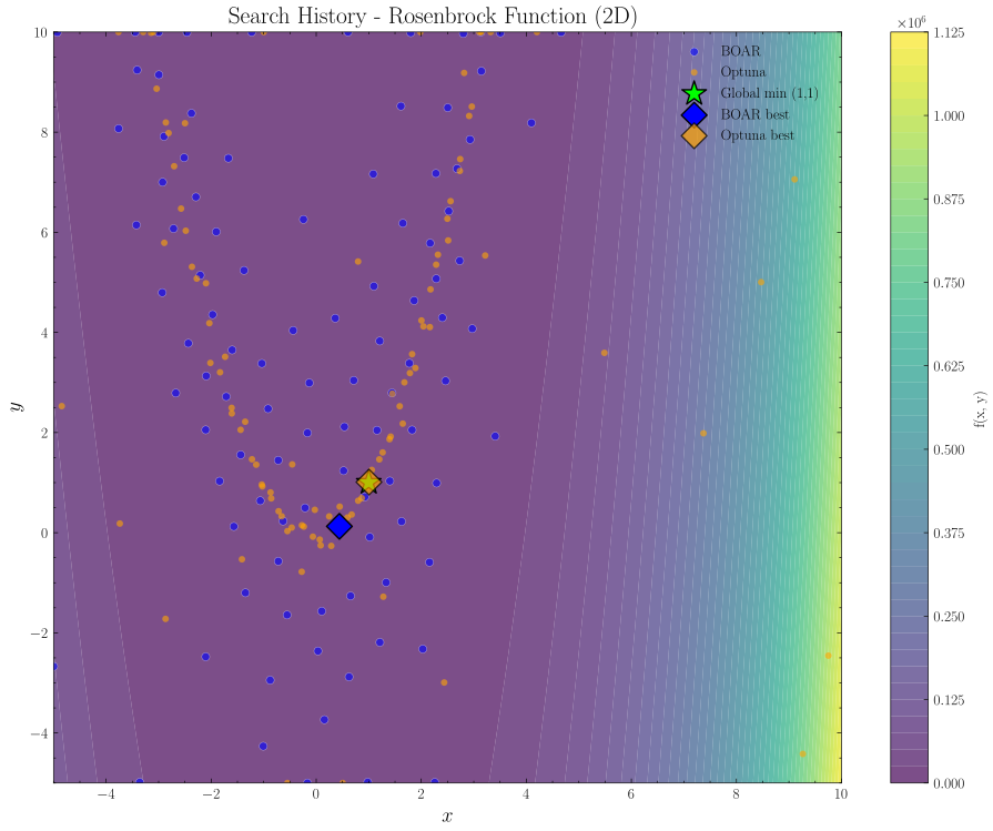
Figure 12: Search history of BOAR optimization on the 2D Rosenbrock function.

Constrained version

The Rosenbrock function can also be tested with constraints, such as limiting the search space to a specific region or adding inequality constraints. In this test case, we defined the following constraint:

\[g(\mathbf{x}) : \sum_{i=0}^{n-1} x_i^2 > n \cdot 5\]

This constraint defines a hypersphere where the feasible region is outside the sphere with radius \(\sqrt{5n}\). The global minimum at \(\mathbf{x} = (1, 1, \ldots, 1)\) lies inside the forbidden sphere, making this a challenging constrained optimization problem.

Equivalent logical form:

# For n_dim = 2:
variables = ['x0', 'x1']
expr = "x0**2 + x1**2 > 10"    # radius = sqrt(10) ≈ 3.16

# For n_dim = 5:
variables = ['x0', 'x1', 'x2', 'x3', 'x4']
expr = "x0**2 + x1**2 + x2**2 + x3**2 + x4**2 > 25"    # radius = 5

# For n_dim = 10:
expr = "x0**2 + x1**2 + ... + x9**2 > 50"    # radius ≈ 7.07

Constrained Benchmark Results

The red dashed circle marks the constraint boundary \(x_0^2 + x_1^2 = 10\). The shaded red region inside the circle is infeasible (inside the forbidden sphere). The feasible region is the entire domain outside the circle.

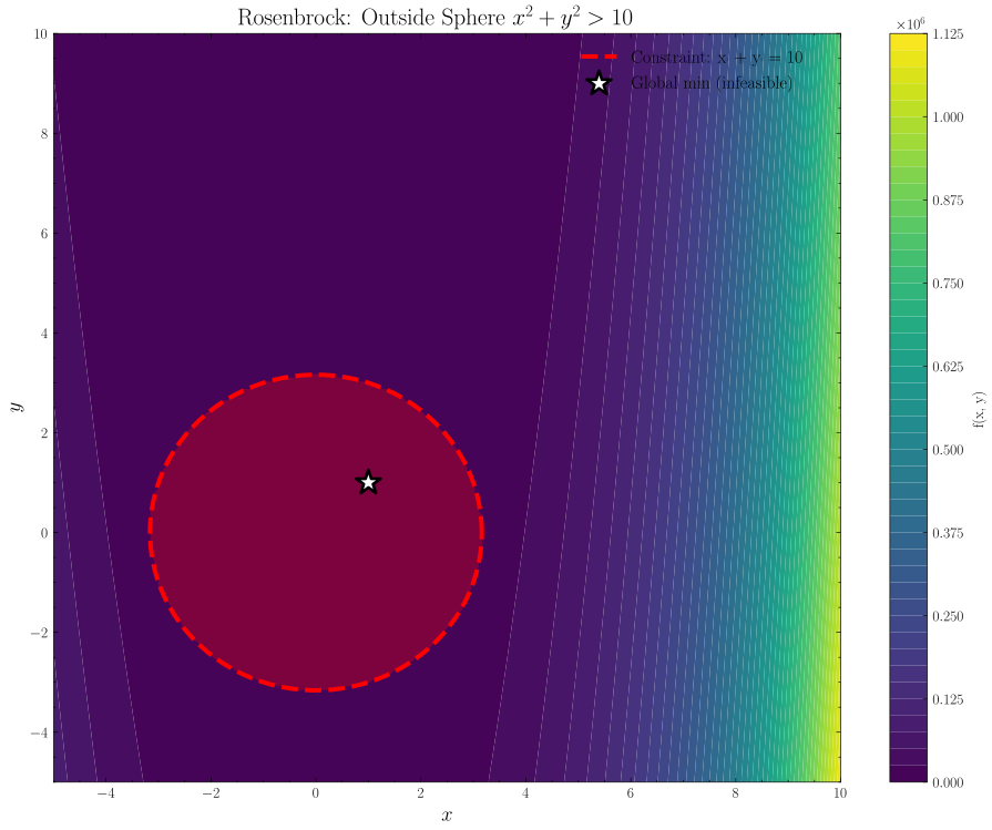
Figure 13: Contour plot of the 2D constrained Rosenbrock function showing feasible region.

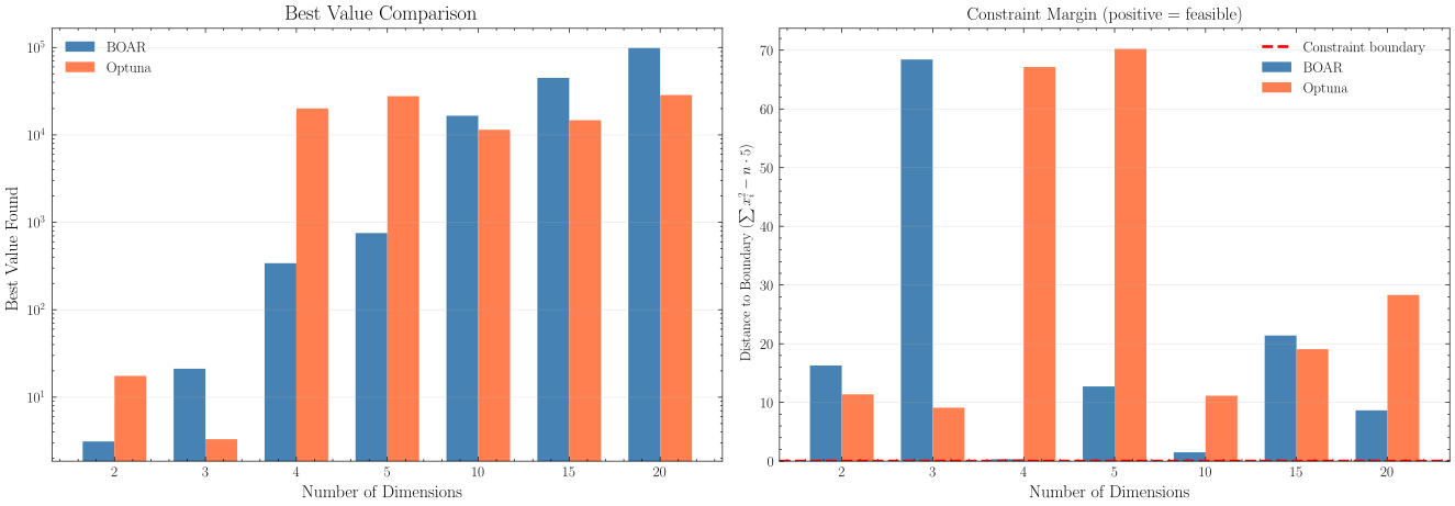
Figure 14: Comparison of available BOAR optimization results on the constrained Rosenbrock function.

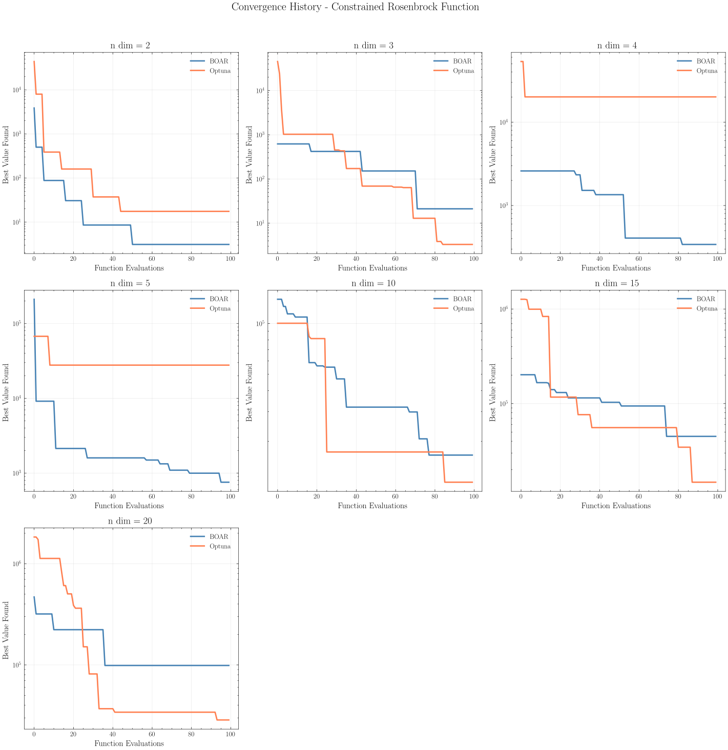
Figure 15: BOAR optimization convergence on the constrained Rosenbrock function.

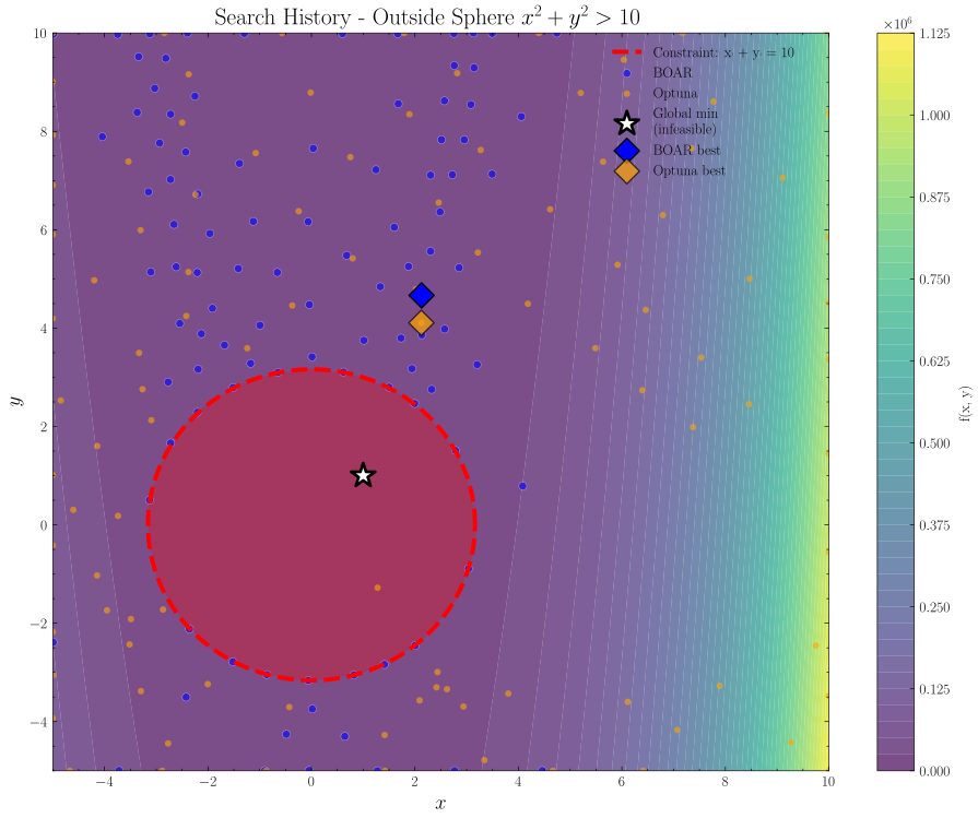
Figure 16: Search history of BOAR optimization on the 2D constrained Rosenbrock function.

Compound Channel Benchmark (BASEMENT v4.2)

A compound channel benchmark is included to demonstrate the framework’s ability to handle a two-dimensional hydrodynamic models calibration. The compound channel was divided into three friction zones (main channel, floodplain, and floodplain forest), each with a different Strickler’s roughness coefficient (Figure 17). The search space for the optimization had 1 dimension (overbank flow), 2 dimensions (main channel and floodplain), 3 dimensions (main channel, floodplain, and floodplain forest), and additional 6-dimensional case was considered, at which the floodplain forest was divided into 4 zones. The goal of the optimization is to calibrate these coefficients to match observed water levels and flow rates.

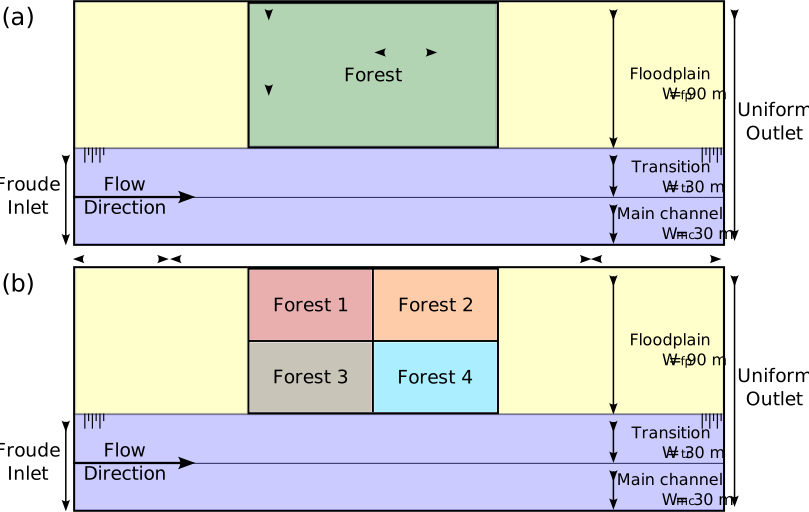
Figure 17: Numerical simulations domain and boundary conditions. (a) For all Bare and Forest scenarions, and (b) artificial dim = 6 scenario applied to the Mid vegetation. Each colour represents a hydraulic roughness region

The loss is computed in terms of the Root Mean Square Error (RMSE) between the observed and simulated water levels and flow rates, normalized by the main channel flow depth. The following conditions were used for the optimization:

optimization_variable_options:
  'bounds': [!!python/tuple [20, 60], !!python/tuple [20, 60], !!python/tuple [10, 35]] # Main channel, Floodplain, Floodplain Forest
  'constraints':
    'expression': "z < x and z < y"  # Floodplain Forest < Main channel and Floodplain
    'variables': ['x', 'y', 'z']
  'precision': 0.1
  'n_initial': 5

surrogate_model_options:
  'max_tested_vectors': 100
  'max_no_improvement': 100
  'tolerance': 1e-4
  'GPR_iterations': 500
  'test_population': 80200

sampling_options:
  'seed': 9

The following results were obtained for the BASEMENT benchmark using the BOAR engine:

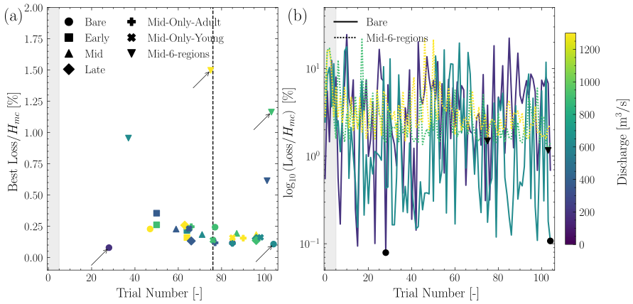
Figure 18: Calibration-convergence analysis based on the normalized \(\mathrm{RMSE}/H_{mc}\): (a) best loss value (%) versus trial number; (b) loss-value trajectories for the Bare and Early cases at the trials highlighted by arrows in panel (a). The dashed line in panel (a) denotes the median number of trials required to obtain the optimal loss, and the black markers in panel (b) indicate the corresponding optimal solution. The shaded light gray area represents the initial training phase. All simulations were performed on a Froude-scaled model at a 1:1 prototype scale.

Note that the convergence is highly tied to the desired tolerance. For instance, if the tolerance is increased to 1.5%, the convergence is achieved in fewer trials (median = 9 trials), as shown in Figure 19.

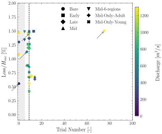
Figure 19: Calibration-convergence analysis based on the normalized \(\mathrm{RMSE}/H_{mc}\) (Loss) versus trial number, with an error threshold of \(\mathrm{Loss}/H_{mc} \leq 1.5\%\). The shaded light gray area represents the initial training phase. All simulations were performed on a Froude-scaled model at a 1:1 prototype scale.

For a more in depth information about the compound channel benchmark, please check de Oliveira et al. (2026) [1].

References

[1]

LED. de Oliveira, MJ. Franca, NP. Huber, D. Vanzo, BOAR: Bayesian Optimization for Automated Roughness calibration in two-dimensional hydrodynamic models. SoftwareX, (under review)